Generative Adverserial Networks
- Deep neural networks are used mainly for supervised learning: classification or regression. Generative Adverserial Networks or GANs, however, use neural networks for a very different purpose, a generative modeling. Generative modeling is an unsupervised learning task in machine learning that involves automatically discovering and learning the regularities or patterns in input data in such a way that the model can be used to generate or output new examples that plausibly could have been drawn from the original dataset.
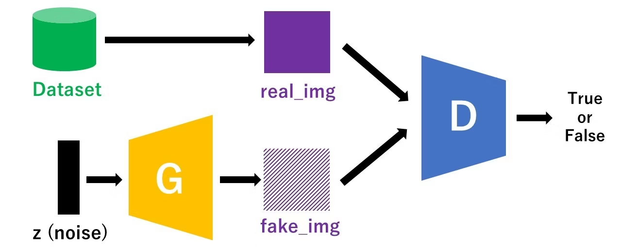
- While there are many approaches used for generative modeling, a Generative Adverserial Network takes the following approach:
- There are two neural networks: a Generator and a Discriminator.
- The generator generates a "fake" sample given a random noise.
- The discriminator attempts to detect whether a given sample is "real" (picked from the training data) or "fake" (generated by the generator).
- Training happens in tandem: we train the discriminator for a few epochs, then train the generator for a few epochs, and repeat. This way both the generator and the discriminator get better at doing their jobs.
- In this tutorial, we'll train a GAN to generate images of handwritten digits. A database for such handwritten digits is called MNIST database, easily and free downloadable. We used this MNIST dataset for traing, and try to generate the MNIST-like handwritten dataset with GAN.
- We'll use the PyTorch library, which is mainly developed Meta. Inc., (previously known as Facebook).
Load the Data
We begin by downloading and importing the data as a PyTorch dataset using the MNIST helper class from
torchvision.datasets.import torch import torchvision from torchvision.transforms import ToTensor, Normalize, Compose from torchvision.datasets import MNIST mnist = MNIST(root='data', train=True, download=True, transform=Compose([ToTensor(), Normalize(mean=(0.5,), std=(0.5,))]))Note that we are are transforming the pixel values from the range [0, 1] to the range [-1, 1]. The reason for doing this will become clear when define the generator network. Let's look at a sample tensor from the data.
img, label = mnist[0]
print('Label: ', label)
print(img[:,10:15,10:15])
torch.min(img), torch.max(img)
Let's plot one of the images.
import matplotlib.pyplot as plt
%matplotlib inline

plt.imshow(img[0], cmap='gray')
plt.show()
print('Label:', label)
Finally, let's create a dataloader to load the images in batches.
from torch.utils.data import DataLoader

batch_size = 100
data_loader = DataLoader(mnist, batch_size, shuffle=True)
We'll also create a device which can be used to move the data and models to a graphical procssing unit (GPU), if one is available. Using GPU is faster than using CPU!
# Device configuration
device = torch.device('cuda' if torch.cuda.is_available() else 'cpu')
Discriminator Network
- The discriminator takes an image as input, and tries to classify it as "real" or "generated". In this sense, it's like any other neural network. While we can use a complicated neural networks, we'll use a simple one with 3 layers.
Since the MNIST image has 28 pixels in width and height, it is 28x28 = 784 pixels. We'll transform it to a vector of size 784.
image_size = 784
hidden_size = 256
import torch.nn as nn

D = nn.Sequential(
    nn.Linear(image_size, hidden_size),
    nn.LeakyReLU(0.2),
    nn.Linear(hidden_size, hidden_size),
    nn.LeakyReLU(0.2),
    nn.Linear(hidden_size, 1),
    nn.Sigmoid())
We use the Leaky ReLU activation for the discriminator. Different from the regular ReLU function, Leaky ReLU allows the pass of a small gradient signal for negative values. As a result, it makes the gradients from the discriminator flows stronger into the generator. Instead of passing a gradient (slope) of 0 in the back-prop pass, it passes a small negative gradient.
Just like any other binary classification model, the output of the discriminator is a single number between 0 and 1, which can be interpreted as the probability of the input image being fake i.e. GAN-generated.
After defineing the discriminator, let's move the model to the chosen device.
D.to(device)
Generator Network
The input to the generator is typically a vector of random noise. Once again, to keep things simple, we'll use a neural network with 3 layers, and the output will be a vector of size 784, which can be transformed to a 28x28 pixel image.
latent_size = 64
G = nn.Sequential(
    nn.Linear(latent_size, hidden_size),
    nn.ReLU(),
    nn.Linear(hidden_size, hidden_size),
    nn.ReLU(),
    nn.Linear(hidden_size, image_size),
    nn.Tanh())
We use the hyperbolic tangent (tanH) activation function for the output layer of the generator.
Let's generate an output vector using the generator and view it as an image by transforming and denormalizing the output.
y = G(torch.randn(2, latent_size))
gen_imgs = y.reshape((-1, 28,28)).detach()
plt.imshow(gen_imgs[0], cmap='gray')
plt.show()
Now move the generator to the chosen device.
G.to(device)
Discriminator Training
Since the discriminator is a binary classification model, we can use the binary cross entropy loss function to quantify how well it is able to differentiate between real and generated images.
criterion = nn.BCELoss()
d_optimizer = torch.optim.Adam(D.parameters(), lr=0.0002)
Let's define helper functions to reset gradients and train the discriminator.
def reset_grad():
    d_optimizer.zero_grad()
    g_optimizer.zero_grad()

def train_discriminator(images):
    # Create the labels which are later used as input for the BCE loss
    real_labels = torch.ones(batch_size, 1).to(device)
    fake_labels = torch.zeros(batch_size, 1).to(device)

    # Loss for real images
    outputs = D(images)
    d_loss_real = criterion(outputs, real_labels)
    real_score = outputs

    # Loss for fake images
    z = torch.randn(batch_size, latent_size).to(device)
    fake_images = G(z)
    outputs = D(fake_images)
    d_loss_fake = criterion(outputs, fake_labels)
    fake_score = outputs

    # Combine losses
    d_loss = d_loss_real + d_loss_fake
    # Reset gradients
    reset_grad()
    # Compute gradients
    d_loss.backward()
    # Adjust the parameters using backprop
    d_optimizer.step()

    return d_loss, real_score, fake_score
Here are the steps involved in training the discriminator.
- We expect the discriminator to output 1 if the image was picked from the real MNIST dataset, and 0 if it was generated.
- We first pass a batch of real images, and compute the loss, setting the target labels to 1.
- Then we generate a batch of fake images using the generator, pass them into the discriminator, and compute the loss, setting the target labels to 0 (fake).
- Finally we add the two losses and use the overall loss to perform gradient descent to adjust the weights of the discriminator.
It's important to note that we don't change the weights of the generator model while training the discriminator (
d_optimizeronly affects theD.parameters())
Generator Training
- Since the outputs of the generator are images, it's not obvious how we can train the generator. This is where we employ a rather elegant trick, which is to use the discriminator as a part of the loss function.
- Here's how it works: We generate a batch of images using the generator, pass the into the discriminator.
- We calculate the loss by setting the target labels to 1 i.e. real. We do this because the generator's objective is to "fool" the discriminator.
We use the loss to perform gradient descent i.e. change the weights of the generator, so it gets better at generating real-like images.
Here's what this looks like in code.
g_optimizer = torch.optim.Adam(G.parameters(), lr=0.0002)
def train_generator():
    # Generate fake images and calculate loss
    z = torch.randn(batch_size, latent_size).to(device)
    fake_images = G(z)
    labels = torch.ones(batch_size, 1).to(device)
    g_loss = criterion(D(fake_images), labels)

    # Backprop and optimize
    reset_grad()
    g_loss.backward()
    g_optimizer.step()
    return g_loss, fake_images
Training the Model
Let's create a directory where we can save intermediate outputs from the generator to visually inspect the progress of the model
import os

sample_dir = 'samples'
if not os.path.exists(sample_dir):
    os.makedirs(sample_dir)
Let's save a batch of real images that we can use for visual comparision while looking at the generated images.
from IPython.display import Image
from torchvision.utils import save_image

# Save some real images
for images, _ in data_loader:
    images = images.reshape(images.size(0), 1, 28, 28)
    save_image(images, os.path.join(sample_dir, 'real_images.png'), nrow=10)
    break

Image(os.path.join(sample_dir, 'real_images.png'))
We'll also define a helper function to save a batch of generated images to disk at the end of every epoch. We'll use a fixed set of input vectors to the generator to see how the individual generated images evolve over time as we train the model.
sample_vectors = torch.randn(batch_size, latent_size).to(device)

def save_fake_images(index):
    fake_images = G(sample_vectors)
    fake_images = fake_images.reshape(fake_images.size(0), 1, 28, 28)
    fake_fname = 'fake_images-{0:0=4d}.png'.format(index)
    print('Saving', fake_fname)
    save_image(fake_images, os.path.join(sample_dir, fake_fname), nrow=10)

# Before training
save_fake_images(0)
Image(os.path.join(sample_dir, 'fake_images-0000.png'))
We are now ready to train the model. In each epoch, we train the discriminator first, and then the generator.
The training might take a while if you're not using a GPU.
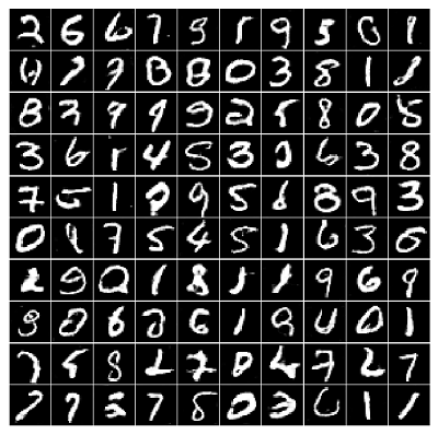
num_epochs = 20
total_step = len(data_loader)
d_losses, g_losses, real_scores, fake_scores = [], [], [], []

for epoch in range(num_epochs):
    for i, (images, _) in enumerate(data_loader):
        # Load a batch & transform to vectors
        images = images.reshape(batch_size, -1).to(device)

        # Train the discriminator and generator
        d_loss, real_score, fake_score = train_discriminator(images)
        g_loss, fake_images = train_generator()

        # Inspect the losses
        if (i+1) % 200 == 0:
            d_losses.append(d_loss.item())
            g_losses.append(g_loss.item())
            real_scores.append(real_score.mean().item())
            fake_scores.append(fake_score.mean().item())
            print('Epoch [{}/{}], Step [{}/{}], d_loss: {:.4f}, g_loss: {:.4f}, D(x): {:.2f}, D(G(z)): {:.2f}'
                  .format(epoch, num_epochs, i+1, total_step, d_loss.item(), g_loss.item(),
                          real_score.mean().item(), fake_score.mean().item()))

    # Sample and save images
    if (epoch+1) % 5 == 0:
        save_fake_images(epoch+1)
Here's how the generated images look, after the 10th, 50th, 100th and 300th epochs of training.
Image('./samples/fake_images-0050.png')
Image('./samples/fake_images-0100.png')
Image('./samples/fake_images-0300.png')
We can also visualize how the loss changes over time. Visualizing losses is quite useful for debugging the training process. For GANs, we expect the generator's loss to reduce over time, without the discriminator's loss getting too high.
plt.plot(d_losses, '-')
plt.plot(g_losses, '-')
plt.xlabel('epoch')
plt.ylabel('loss')
plt.legend(['Discriminator', 'Generator'])
plt.title('Losses')
plt.show()